set.seed(2023)
x <- round(runif(20,1,15),2)
y <- 20+5*x + rnorm(20,0,2)*x해당 자료는 전북대학교 이영미 교수님 2023응용통계학 자료임
WLSE
- 등분산성을 만족하지 않을 때! 하자
\(N(0,2)x \rightarrow N(0,2x^2)\)
\(Var(\epsilon)= \sigma^2\)이 \(x^2\)에 비례
plot(y~x, pch=16)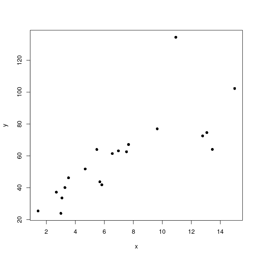
- X가 커지면서 분산도 커진다..
m <- lm(y~x)
m1 <- lm(y~x, weights = 1/x^2)
\(Var(\epsilon) = \dfrac{\sigma^2}{w_i}=x^2 \sigma^2\)
\(w_i = \dfrac{1}{x^2}\)
LSE는 \(argmin \sum_{i=1}^n(y_i-\hat y_i)^2\)
WLSE는 잔차 가중치의 제곱합을 가장 작게 해주는..
WLSE: \(argmin \sum_{i=1}^n w_i (y_i - \hat y_i)^2\)
MSE관점에서 더 좋은 추정량
- LSE
summary(m)
Call:
lm(formula = y ~ x)

Residuals:
    Min      1Q  Median      3Q     Max
-27.007  -9.123   0.579   4.872  55.973

Coefficients:
            Estimate Std. Error t value Pr(>|t|)
(Intercept)  23.7109     7.7116   3.075  0.00653 **
x             5.0099     0.9461   5.295 4.92e-05 ***
---
Signif. codes:  0 ‘***’ 0.001 ‘**’ 0.01 ‘*’ 0.05 ‘.’ 0.1 ‘ ’ 1

Residual standard error: 16.83 on 18 degrees of freedom
Multiple R-squared:  0.609, Adjusted R-squared:  0.5873
F-statistic: 28.04 on 1 and 18 DF,  p-value: 4.924e-05
- WLSE
summary(m1)
Call:
lm(formula = y ~ x, weights = 1/x^2)

Weighted Residuals:
    Min      1Q  Median      3Q     Max
-3.8348 -1.4757  0.0365  1.0085  4.6530

Coefficients:
            Estimate Std. Error t value Pr(>|t|)
(Intercept)  17.1950     3.0315   5.672 2.22e-05 ***
x             6.0742     0.7657   7.933 2.76e-07 ***
---
Signif. codes:  0 ‘***’ 0.001 ‘**’ 0.01 ‘*’ 0.05 ‘.’ 0.1 ‘ ’ 1

Residual standard error: 1.99 on 18 degrees of freedom
Multiple R-squared:  0.7776,    Adjusted R-squared:  0.7653
F-statistic: 62.94 on 1 and 18 DF, p-value: 2.761e-07par(mfrow=c(1,1))
plot(x,y,pch=16)
abline(m, col='red', lwd=2)
abline(m1, col='blue', lwd=2)
legend("topleft",c('OLS', "WLS"), lty=1,
col=c('red', 'blue'), lwd=2)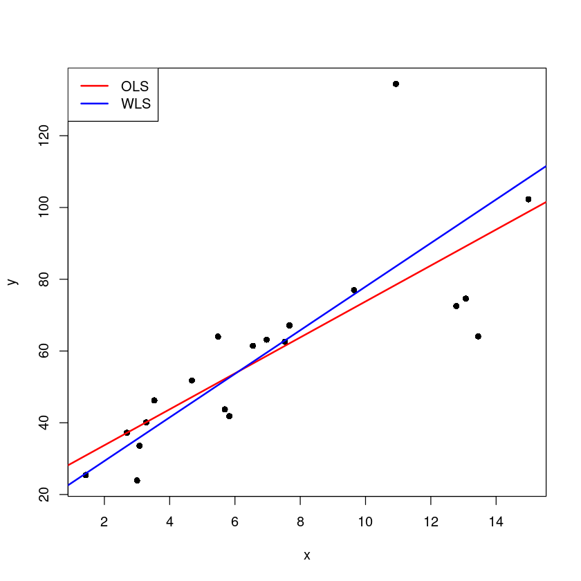
par(mfrow=c(1,2))
plot(fitted(m), resid(m),pch=16,xlab=expression(hat(y)), ylab=expression(e[i]),main="OLS")
abline(h=0)
plot(fitted(m)/x, resid(m)/x,pch=16,xlab=expression(sqrt(w[i])*hat(y)), ylab=expression(sqrt(w [i])*e[i]), main="WLS")
abline(h=0)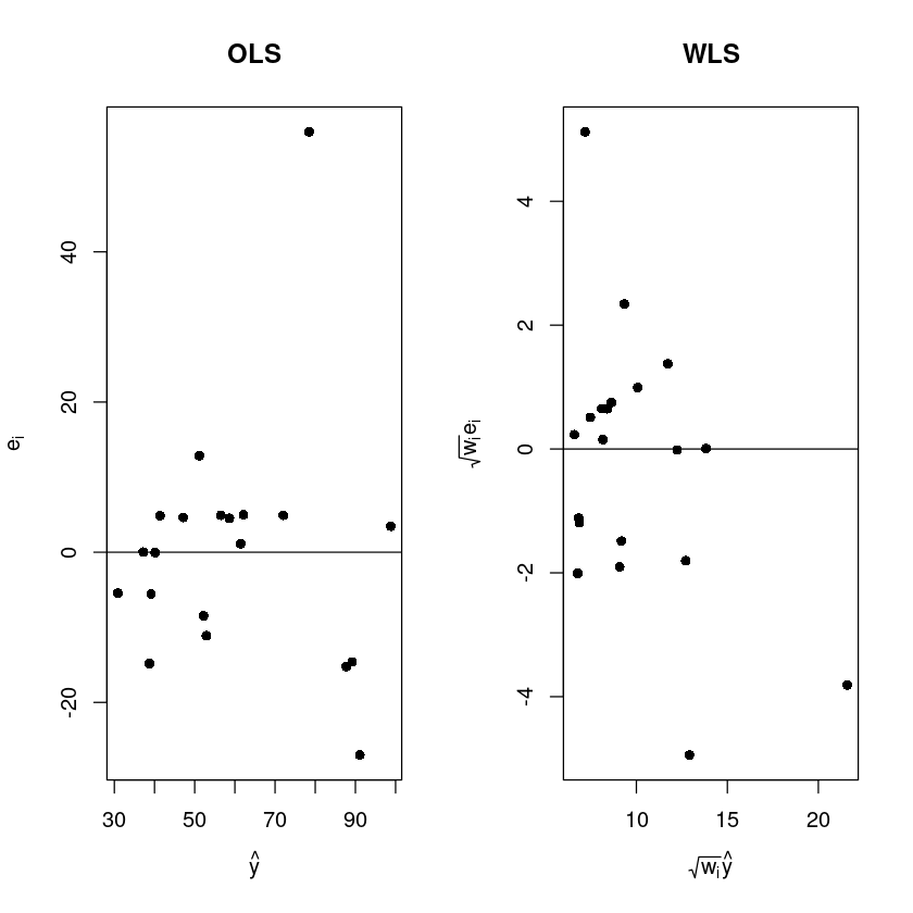
OLS는 퍼져 있다.
WLS는 \(\sqrt{w_i}y_i = \sqrt{w_i}\beta_0 + \sqrt{w_i}\beta_1x_i + \sqrt{w_i} \epsilon_i\)
\(\sqrt{w_i} \epsilon_i\) ~ \(N(0,2)\)
\(\sqrt{w_i} y_i = \hat y' = \beta_0' + \beta_1 x_i' + \epsilon_i'\)
분산이 어느정도 안정화 됭
- OLS (LSE)
y = X \(\beta\) + \(\epsilon\)
\(\epsilon\) ~ \(N(0_n, In\sigma^2)\)
\(\hat \beta = (X^TX)^{-1}X^Ty\)
- GLS (WLSE)
y = X \(\beta\) + \(\epsilon\)
\(Var(\epsilon) = V\sigma^2\)
\(\hat \beta^{G} = (X^TV^{-1}X)^{-1}X^TV^{-1}y\)
V<-diag(x^2)
X<-model.matrix(m)
V.inv<-solve(V)
beta<-solve(t(X)%*%V.inv%*%X)%*%t(X)%*%V.inv%*%y
beta | (Intercept) | 17.194962 |
| x | 6.074163 |
summary(m1)$coef| Estimate | Std. Error | t value | Pr(>|t|) | |
|---|---|---|---|---|
| (Intercept) | 17.194962 | 3.0314900 | 5.672116 | 2.220897e-05 |
| x | 6.074163 | 0.7656541 | 7.933298 | 2.760514e-07 |
\(lm(y\) ~ \(x, wieght=\frac{1}{x^2})\)
GLS구한거랑 WLS로 구한거랑 6.074163 값 동일
e2 <- y-(beta[1]+beta[2]*x)
t(e2) %*% V.inv %*%e2 | 71.26588 |
anova(m1)| Df | Sum Sq | Mean Sq | F value | Pr(>F) | |
|---|---|---|---|---|---|
| <int> | <dbl> | <dbl> | <dbl> | <dbl> | |
| x | 1 | 249.18204 | 249.182044 | 62.93722 | 2.760514e-07 |
| Residuals | 18 | 71.26588 | 3.959216 | NA | NA |
1차 자기상관 회귀모형
- 독립성을 만족하지 않을 때! 하자
dt <- read.csv("corr.csv")
head(dt)| y | x | |
|---|---|---|
| <dbl> | <dbl> | |
| 1 | 349.7 | 133.6 |
| 2 | 353.5 | 135.4 |
| 3 | 359.2 | 137.6 |
| 4 | 366.4 | 140.0 |
| 5 | 376.5 | 143.8 |
| 6 | 385.7 | 147.1 |
plot(y~x, dt, pch=16)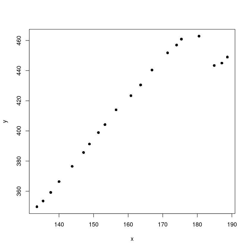
- 오른쪽 4개 데이터가 애매하다.
m <- lm(y~x, dt)- \(y=\beta_0+\beta_x + \epsilon\)
summary(m)
Call:
lm(formula = y ~ x, data = dt)

Residuals:
    Min      1Q  Median      3Q     Max
-22.959  -8.874   2.035   9.035  16.623

Coefficients:
            Estimate Std. Error t value Pr(>|t|)
(Intercept)   89.234     26.721   3.339  0.00365 **
x              2.024      0.166  12.196 3.89e-10 ***
---
Signif. codes:  0 ‘***’ 0.001 ‘**’ 0.01 ‘*’ 0.05 ‘.’ 0.1 ‘ ’ 1

Residual standard error: 12.98 on 18 degrees of freedom
Multiple R-squared:  0.892, Adjusted R-squared:  0.886
F-statistic: 148.7 on 1 and 18 DF, p-value: 3.888e-10par(mfrow=c(1,1))
plot(dt$x, resid(m), pch=16)
abline(h=0)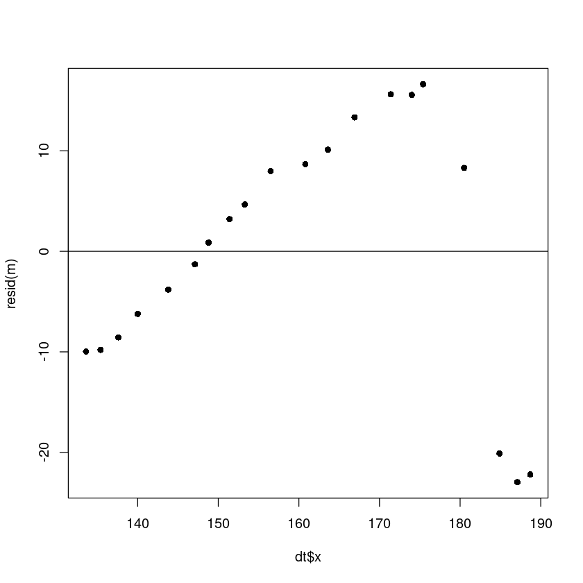
library(lmtest)Loading required package: zoo
Attaching package: ‘zoo’
The following objects are masked from ‘package:base’:
as.Date, as.Date.numeric
dwtest(m)
    Durbin-Watson test

data:  m
DW = 0.31237, p-value = 1.238e-08
alternative hypothesis: true autocorrelation is greater than 0
DW값이 0에 가까우므로 양의상관관계를 가진다.
2에 가까우면 상관관계가 0에 가까움
4에 가까우면 음의 상관관계에 가까움
plot(y~x, dt, pch=16)
abline(m, col='darkorange', lwd=2)
legend("topleft", "OLS",col="darkorange", lty=1)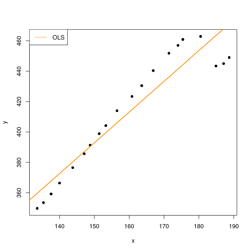
plot(fitted(m), resid(m), pch=16,xlab=expression(hat(y)), ylab='residual',
     main=paste0("residua l plot for OLS : DW statistics = ", round(dwtest(m)$stat,4)))
abline(h=0)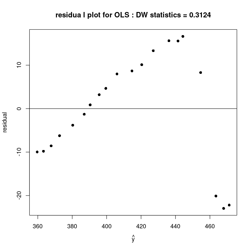
변수변환
bar_e1 <- mean(resid(m)[-1])
bar_e2 <- mean(resid(m)[-20])
# hat_rho <- sum((resid(m)[-1]-bar_e1)*(resid(m)[-20] - bar_e2))/sum((resid(m)[-1]-bar_e1)^2) #일밎게 구하는거
hat_rho <- sum(resid(m)[-1]*resid(m)[-20])/sum((resid(m)[-20])^2)  #대략적으로 구하는거
# hat_rho <- cor(resid(m)[-1], resid(m)[-20])
hat_rho
0.891002040194419
- \(Corr(\epsilon_i, \epsilon_j) \neq 0, i \neq j\)
- 1차 자기상관 회귀모형
\(y=\beta_0 + \beta_1 x + \epsilon\)
\(\epsilon_i = \rho \epsilon_{i-1} + \delta_i\)
\(\delta_i\) ~ \(N(0,\sigma^2), iid\)
현시점의 오차가 다음 시점의 오차에 영향을 준다. ->시계열 데이터와 관련된 모형
\(y_i=\beta_0+\beta_1x_i + \epsilon_i\)
\(\rho y_{i-1} = \beta_0 + \beta_1 \rho x_{i-1} + \rho \epsilon_{i-1}\)
\(y_i - \rho y_{i-1}=(1-\rho)\beta_0 + \beta_1 (x_i - \rho x_{i-1}) + \epsilon_i - \rho \epsilon_{i-1}\)
위를
\(y' = \beta_0' + \beta_1'x_i' + \delta_i\)
\(\hat \rho = \dfrac{\sum_{i=2}^n e_i e_{i-1}}{\sum_{i=2}^n e_i^2}=0.891002040194419\)
y1 <- dt$y[-1]-hat_rho*dt$y[-20]
x1 <- dt$x[-1]-hat_rho*dt$x[-20]
m1 <- lm(y1~x1)
summary(m1)
Call:
lm(formula = y1 ~ x1)

Residuals:
     Min       1Q   Median       3Q      Max
-20.9956  -1.2060   0.7668   3.7082   8.1241

Coefficients:
            Estimate Std. Error t value Pr(>|t|)
(Intercept)  40.2455    13.1639   3.057  0.00713 **
x1            0.4862     0.6483   0.750  0.46354
---
Signif. codes:  0 ‘***’ 0.001 ‘**’ 0.01 ‘*’ 0.05 ‘.’ 0.1 ‘ ’ 1

Residual standard error: 6.347 on 17 degrees of freedom
Multiple R-squared:  0.03202,   Adjusted R-squared:  -0.02492
F-statistic: 0.5624 on 1 and 17 DF, p-value: 0.4635dwtest(m1)
    Durbin-Watson test

data:  m1
DW = 1.3704, p-value = 0.04663
alternative hypothesis: true autocorrelation is greater than 0- 데이터가 많지 않아서 크게 dw가 차이나지 ㄴ않음..
par(mfrow=c(1,1))
plot(y1~x1,pch=16,  xlab=expression(x^"'"),  ylab=expression(y^"'"),
     main="scatter plot after v ariable transformation")
abline(m1, col='darkorange', lwd=2)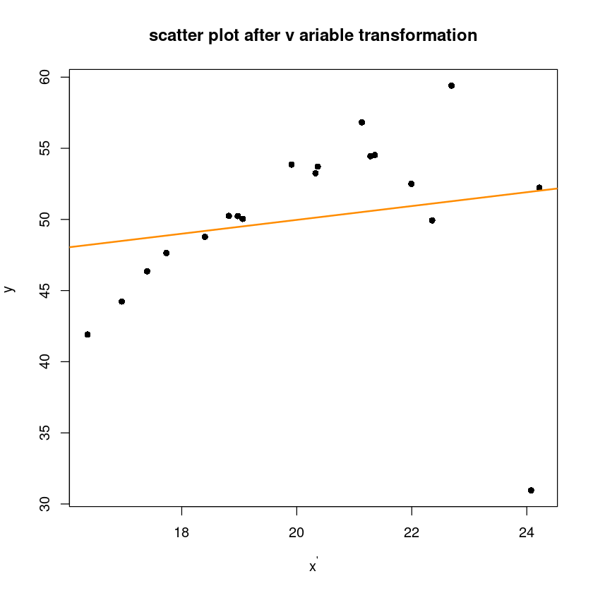
plot(fitted(m1), resid(m1), pch=16,xlab=expression(hat(y)), ylab='residual',
     main=paste0("residual plot for OLS : DW statistics = ", round(dwtest(m1)$stat,4)))
abline(h=0)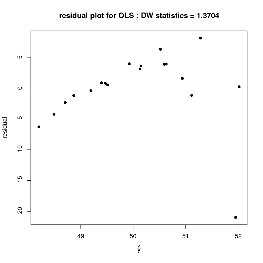
GLS
V<-diag(20)
V<-hat_rho^abs(row(V)-col(V))
X<-model.matrix(m)
V.inv<-solve(V)
beta<-solve(t(X)%*%V.inv%*%X)%*%t(X)%*%V.inv%*%dt$y
beta| (Intercept) | 131.745681 |
| x | 1.714326 |
plot(y~x, dt, pch=16)
abline(m, col='darkorange', lwd=2)
abline(beta[1], beta[2], col='steelblue', lwd=2)
legend("topleft", c("OLS", "GLS"),col=c("darkorange", 'steelblue'), lty=1, lwd=2)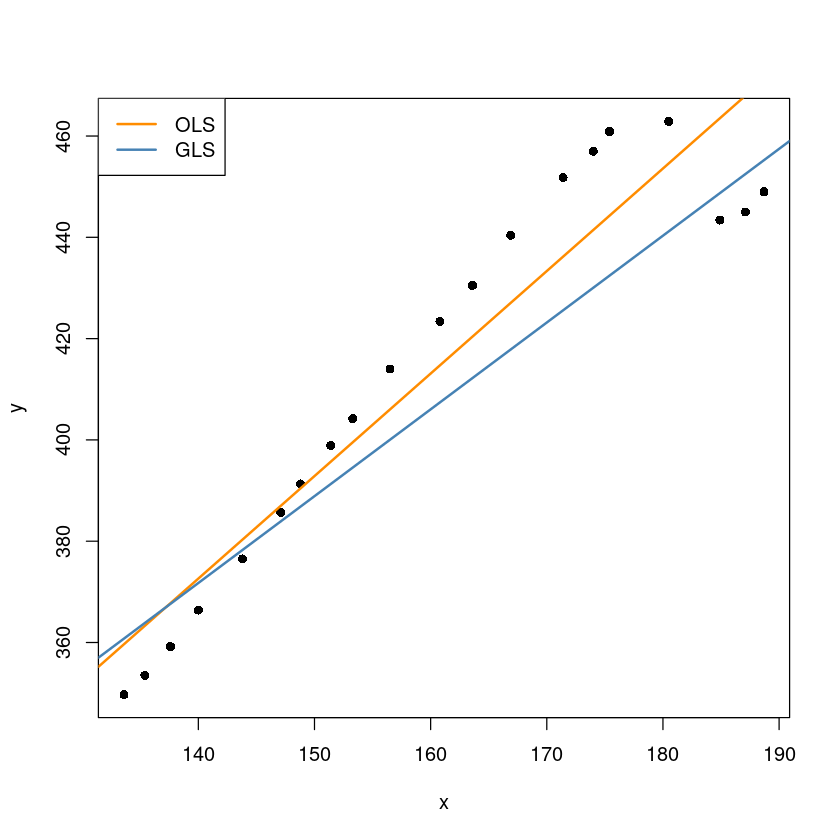
- 시간 변수를 더 추가해보자.
dt$t <- 1:nrow(dt)

m2 <- lm(y~t, dt)
summary(m2)
Call:
lm(formula = y ~ t, data = dt)

Residuals:
    Min      1Q  Median      3Q     Max
-23.107  -6.594   0.372   8.359  16.907

Coefficients:
            Estimate Std. Error t value Pr(>|t|)
(Intercept) 348.0605     5.4652   63.69  < 2e-16 ***
t             6.2023     0.4562   13.60  6.6e-11 ***
---
Signif. codes:  0 ‘***’ 0.001 ‘**’ 0.01 ‘*’ 0.05 ‘.’ 0.1 ‘ ’ 1

Residual standard error: 11.77 on 18 degrees of freedom
Multiple R-squared:  0.9113,    Adjusted R-squared:  0.9063
F-statistic: 184.8 on 1 and 18 DF, p-value: 6.605e-11summary(m)
Call:
lm(formula = y ~ x, data = dt)

Residuals:
    Min      1Q  Median      3Q     Max
-22.959  -8.874   2.035   9.035  16.623

Coefficients:
            Estimate Std. Error t value Pr(>|t|)
(Intercept)   89.234     26.721   3.339  0.00365 **
x              2.024      0.166  12.196 3.89e-10 ***
---
Signif. codes:  0 ‘***’ 0.001 ‘**’ 0.01 ‘*’ 0.05 ‘.’ 0.1 ‘ ’ 1

Residual standard error: 12.98 on 18 degrees of freedom
Multiple R-squared:  0.892, Adjusted R-squared:  0.886
F-statistic: 148.7 on 1 and 18 DF,  p-value: 3.888e-10